CE740 (3 0 1 8) - Traffic Engineering
Autumn 2013
Printer friendly page
End Sem Key
Introduction, Basic for traffic engineering; Planning and design of facilities;
Travel forecasting principles and techniques; Design Hourly volumes and speed;
Highway capacity and performance characteristics; Parking, simulation in
Traffic engineering design.
See detailed lecture list
See the current time table
Best time to meet me: after the class.
| Quizzes |
10.0 |
open notes, surprise |
| Assignments |
12.5 |
including Excel |
| Mid Sem |
20.0 |
closed notes |
| Term paper |
07.5 |
report and presentation |
| Lab class |
15.0 |
report (by TAs) |
| Lab viva |
10.0 |
|
| End Sem |
25.0 |
closed notes |
| Total |
100 |
|
The weights may be changed (plus or minus 5 percent).
- See the lecture notes page
To be handled by TA's
Instructions:
Maintain a separate note book for assignments.
All questions must be hand written.
Start new question on a new page.
Descriptive questions should be rich in figures/tables/equations along with appropriate references (books/journals).
Student shall do this assignments independently.
Submit the assignment on Friday's to the TA who will sign and give you back.
Evaluation by the instructor will be done randomly.
Copying, if found, will have grade penalty.
-
Select a current transportation issue for modeling and do the following.
(i) Identify the transportation system components,
(ii) Activity system that is interest to the transportation issue,
(iii) What could be a suitable service function,
(iv) What could be a suitable demand function,
(v) Visualize how the activity system may change,
(vi) Propose some transport improvement options,
(vii) Illustrate flow predictions.
(D/L Aug 09)
-
Draw a typical time-distance diagram of a non-unform flow and illustrate the concept of flow and density measurement.
(D/L Aug 09)
-
Derive the relationship between the time mean speed and space mean speed.
Verify the above relation using some hypothetical speed data expressed in a frequency table.
(D/L Aug 09)
-
Show the functional form and illustration of any traffic stream model (other than the ones covered in the class).
Give the reference from where it has taken.
(D/L Aug 09)
-
If we assume that drivers keep a gap of one car length for each 10 kmph
increment of the speed and if the car length is 6 meters, develop the equations
of stream flow and draw the fundamental diagrams.
[Hint: write expression for gap interms of speed. density is inverse of gap.]
(D/L Aug 09)
-
The table given below shows headway data for a number of traffic conditions.
It is assumed that the traffic contains only cars and trucks.
Compute the PCU values using the headway method for each traffic condition and
plot how the PCU values changes with respect to the percentage of trucks.
| Average headway for mixed traffic |
Headway for traffic consisting of cars only |
percentage of trucks |
| 2.7 |
2.5 |
0.1 |
| 2.8 |
2.5 |
0.15 |
| 2.94 |
2.5 |
0.2 |
| 3.1 |
2.5 |
0.25 |
| 3.25 |
2.5 |
0.3 |
| 3.35 |
2.5 |
0.35 |
| 3.7 |
2.5 |
0.5 |
| 3.8 |
2.5 |
0.55 |
| 3.95 |
2.5 |
0.6 |
| 4.2 |
2.5 |
0.7 |
(D/L Aug 09)
-
Write a brief note on the following:
(A) One example of intrusive method of data collection,
(B) One example of non-intrusive technology,
(C) One example of in-vehicle technology.
The write up should be organized under these heads: (i) working principle
(supported with simple sketches), (ii) Advantages and disadvantages, (iii) any
Traffic application, (iv) Commercial product details (any one company), and (v) Reference.
Item i-iii should be from good books/reports and (iv) from company website.
Devote about 2-4 page per technology.
(D/L Aug 14)
-
Derive the fundamental macroscopic relations between q, k, and v, if we assume Forbe's car following behaviors.
For some assumed reaction time and vehicle length, compute the boundary conditions.
(D/L Aug 23)
-
Write a 2-3 page note on the car-follwing model used in VISSIM traffic simulator.
(D/L Aug 23)
-
Generate about 30 to 50 arbitrary random head ways such that their maximum is less then 10 seconds, minimum is more than 0.5 seconds and mean should be between 3 and 5 seconds.
Represent the above headway in a frequency table (0.5 or 1.0 second interval).
Discuss the relative merit and demerits of exponential, normal, and Person distribution with various statistics.
Make suitable assumptions for required constants.
The hand calculations must be shown.
(D/L Sep 10)
-
The traffic flow data on given intersection is as follows:
E-W flow is Through 710, Left 284, Right 426;
W-E flow is Through 575, Left 230, Right 345;
N-S flow is Through 320, Left 128, Right 192; and
S-N flow is Through 290, Left 116, Right 174 vehicles per hour.
Given that for all the phases the yellow time is 4 seconds, the lost time is
3 seconds, saturation headway 2.2 seconds, and degree of saturation is 0.9.
The left turn adjustment factor 1.2 and right turn adjustment factor 1.4.
Given that E-W corridor has four lanes each and N-S has two lanes.
Assume: a reasonable saturation headway, there is no pedestrian requirement,
and free left turn where ever possible.
Design the signal for all the three phase plan options (four phase system) and
recommend the system that gives minimum intersection delay.
(D/L Sep 10)
Instructions.
These assignments has to be done on any spread sheet (Excel/Open office etc.).
Each student has to create his/her assignment from scratch.
Each student has to create a drop-box account and create a public folder with name rollno name and share ONLY with the instructor.
Each assignment will be uploaded on or before the deadline.
You have to follow the strict file name convention.
Each file will start with your roll no, followed by the assignment no, followed by an experiment name, followed by version no (starting with 1).
Dropbox folder will show the upload date and will be used to check late submission.
If you made a mistake in a file and and would like to correct, the corrected file should be uploaded with same name but with version 2 and so on.
Each excel file should have only one sheet.
- Write a program to compute the time mean and space mean speed from a frequency table and verify their relationship.
File name rollno_01_meanspeed_v_x.xlsx where rollno is your roll number, and x is the version no (1,2,3, etc.).
(D/L Aug 07)
- Write a program to calibrate greenshields model given several speed density values.
The program should calculate all the parameters and boundary conditions.
Also plot the fundamental diagram.
File name rollno_02_greenshields_v_x.xlsx where rollno is your roll number, and x is the version no (1,2,3, etc.).
(D/L Aug 12)
- Write a program to compute the following speed statistics: mean, median,
Nth percentile (N should be any value between 0 and 100), quartiles, SD, and
standard error of the mean from a frequency table.
The program should also plot the speed histogram, frequency distribution curve, and cumulative frequency distribution curve.
File name rollno_03_speedstat_v_x.xlsx where rollno is your roll number, and x is the version no (1,2,3, etc.).
(D/L Aug 14)
- Illustrate the performance of traffic stream models (v-k relation)
such as Greenberg, Greenshield, Underwood, Pipes, Forbes for some arbitrary boundary conditions.
File name rollno_04_streammodels_v_x.xlsx where rollno is your roll number, and x is the version no (1,2,3, etc.).
(D/L Aug 21)
- Write a program to demonstrate the General motors car-following model (GM5).
The program should work for any acceptable values of sensitivity coefficient, speed exponent, and spacing exponent.
Assume an update interval of 0.1, 0.2, 0.3 or 0.4 and a reaction time of 0.8, 0.9, or 1.2
The program should also plot the velocity and acceleration profile of the lead and following vehicles.
File name rollno_05_carfollowing_v_x.xlsx where rollno is your roll number, and x is the version no (1,2,3, etc.).
(D/L Aug 21)
- Write a program in excel (sheet 1) to generate random head ways given any
flow rate between 500 and 3000 vehicle per hour (generate at least 1000 samples).
In sheet 2, translate the data into a frequency table (0.5 second range) and fit exponential, normal and Person distribution.
Program should take alpha (for normal and person) and K value (for person) as user input.
Sheet 3, should evaluate all the distribution by computing mean, SD, Chi-square value, and comparative plot.
File name rollno_06_distributions_v_x.xlsx where rollno is your roll number, and x is the version no (1,2,3, etc.).
(D/L Sep 10 )
- Write a program to do signal design and evaluation.
Assume four arm junction with a fixed phase plan (either free left or part of a
phase).
The user input includes: all flows, saturation headway for each phase, lost
time for each phase, and amber time for each phase, degree of saturation,
number of lanes (1, 2, 3, or 4) for each phase.
The program should compute critical flow, cycle time, green time, and delays
for each phase and approach.
The program should be as user friendly as possible.
File name rollno_07_trafficsignal_v_x.xlsx where rollno is your
roll number, and x is the version no (1,2,3, etc.).
(D/L Sep 10 )
- Write a program to do two way signal coordination.
(i) First sheet for two way coordination of two junctions. User input include the link lenght, platoon speed, volume on each direction, cycle, and split.
Assume two phase signal.
(ii) Second sheet for two way coordination of multiple junctions preferably five or more.
User input include the length of each link, split on each junction, the common cycle length, common platoon speed, volume on forward and reverse direction.
File name rollno_08_coordination_v_x.xlsx where rollno is your
roll number, and x is the version no (1,2,3, etc.).
(D/L Oct 01)
- Bring first page print of 5-6 good qaulity journal paper (good citation, h-index) on an interesting research topic in the area of traffic engineering.
(Should be different from your credit seminar topic.).
(D/L Oct 03).
-
The spot speeds of ten vehicles observed at a certain location are 55.1, 40.8,
32.2, 47.8, 64.5, 53.2, 58.2, 66.6, 36.4, and 53.2 kmph. Find (i) the 85th
percentile speed and (ii) the probability that the speed exceeds 85th
percentile assuming that speeds follow a normal distribution.
- Compute the mean
 .
.
- Compute the standard deviation
![$\sigma=\sqrt{[(50.8-55.1)^2+(50.8-40.8)^2+(50.8-32.2)^2+\dots]/10}=10.88$](img2.png) .
.
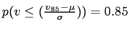
- (i) Since the speed follows normal distribution,
 will correspond to the probability 0.85.
That is:
will correspond to the probability 0.85.
That is:
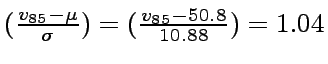
 . Hence,
 corresponding to 0.85 from the standard normal table is 1.04.
In other words,
corresponding to 0.85 from the standard normal table is 1.04.
In other words,
 .
Solving, we get
.
Solving, we get
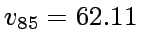 kmph.
(ii) The required probability, by definition, is 1-0.85=0.15.
kmph.
(ii) The required probability, by definition, is 1-0.85=0.15.
An observer counts 300 vehicles in an hour at a location. Assuming that the
vehicle arrival follows Poisson distribution: (i) estimate the probability of 2
or 3 vehicles arriving in a 20-second time interval; and (ii) estimate how many
vehicles will be generated in two minutes (Use the following random numbers:
0.20, 0.92, 0.54, 0.48, 0.69, 0.50, 0.27, 0.57)
- Given
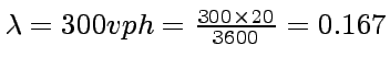 veh per 20
seconds.
veh per 20
seconds.
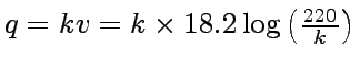
- Using Poisson probability distribution, the following probabilities can be computed:
- Hence, the ans (i): p(x=2 or 3) = p(x=2)+p (x=3) = 0.408.
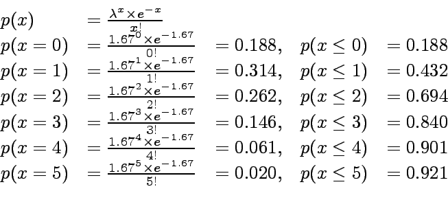
- The interval, random number used and the vehicle generated using the
above results (for two minutes, that is six intervals) are give below:
Note that the first interval, the random number is 0.02 and it is greater than p(0) and less than p(1) and hence, one vehicle is generated.
Similarly, the other intervals.
- Hence, ans (ii) is 14 vehicles per two minutes.
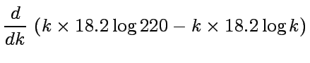
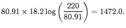
What is the maximum flow and the corresponding density of a traffic stream
whose speed density relationship is given as:
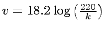
- Since
 , the density
corresponding to maximum flow can be obtained by differentiating with respect
to k and equating to zero.
, the density
corresponding to maximum flow can be obtained by differentiating with respect
to k and equating to zero.
- Hence, Maximum flow is 1472.9 occurring at a density of 80.91.
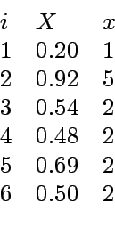
Traffic flow and phase plan for a four-arm intersection is shown in figure below.
The E-W flow is 1420, W-E flow is 1150, N-S flow is 640, and S-N flow is 580
vehicles per hour.
Assume for all the phases the yellow time is 3 seconds, the
lost time is 4 seconds, saturation headway is 1.2 seconds, and degree of
saturation is 0.9.
Assume left turn adjustment factor 1.2 and right turn
adjustment factor 1.3.
Assume left turn and right turn traffic proportions of
20 and 30 percent respectively.
Assuming no pedestrian traffic, compute signal timing
and illustrate with a sketch.
Figure 1:
Intersection Geometry
|
For the above problem, if the actual green time allotted is 30, 28, 18 and 22
respectively for phase 1, 2, 3 and 4, compute the delay for each lane and total
intersection delay.
Download the pdf file
- 1
-
D R Drew.
Traffic flow theory and control.
McGraw-Hill Book Company, New York, 1968.
IITB-.
- 2
-
Highway Capacity Manual.
Transportation Research Board.
National Research Council, Washington, D.C., 2000.
- 3
-
L. R Kadiyali.
Traffic Engineering and Transportation Planning.
Khanna Publishers, New Delhi, 1987.
- 4
-
S K Khanna and C E G Justo.
Highway Engineering.
Nemchand Bros.,, Roorkee, 1991.
- 5
-
M L Manheim.
Fundamentals of transportation systems analysis Vol.1.
MIT Press, 1978.
- 6
-
Adolf D. May.
Fundamentals of Traffic Flow.
Prentice - Hall, Inc. Englewood Cliff New Jersey 07632, second
edition, 1990.
- 7
-
William R McShane, Roger P Roesss, and Elena S Prassas.
Traffic Engineering.
Prentice-Hall, Inc, Upper Saddle River, New Jesery, 1998.
- 8
-
C. S Papacostas.
Fundamentals of Transportation Engineering.
Prentice-Hall, New Delhi, 1987.
- 9
-
M Whol and B V Martin.
Traffic system analysis for engineers and planners.
McGraw Hill, Inc., 1983.
Prof. Tom V. Mathew
2013-12-03
![$\displaystyle 18.2 \log 220 - \left[18.2 k \frac{1}{k}+18.2 \log k \right]$](img16.png)


![\includegraphics[width=6cm]{1506}](img24.png)