
Regression AnalysisTrip Generatrion
Theory
Regression Models Single Linear Regression Model (SLRM)Given a scattered figure shown in Figure 2 it is assumed that the relation between the dependent variable $Y$ and independent variable $X$ is linear. The method of least squares linear regression can be used to find one straight line that fits best for the given scattered diagram. We know that there can be infinite number of such lines each having a unique pair of $Y$ intercept $a$ and slope $b$. Hence our problem is reduced in finding these two variables $a$ and $b$ that defines the best fitting straight line.
An example below will give you an idea about the Regression Model with only one independent variable x
| Y Values | X Values |
|---|---|
| 0.3415 | 0.7 |
| 0.50705 | 0.89 |
| 0.648 | 1.2 |
| 0.5554 | 1.32 |
| 0.514 | 1.2 |
| 1.135 | 3 |
| 0.9245 | 2.1 |
The Values of a and b should be selected such that the Linear Equation (1) will best represent the table above.
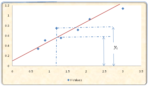
For $i^{th}$ observation $x_i$ let $y_i$ be the observed value and the corresponding estimated value obtained from equation (1) be denoted as $y_e$. The difference between them is called as error, deviation or residual. A best fit curve in our line is obtained only when this error is minimum. Thus to remove the positive and negative signs, sum of squares of error is taken which is minimised and the corresponding value of $a$ and $b$ is found out.
$$\nonumber S =\sum\limits_{i=1}^N (y_i - y_e)^2$$ $$\nonumber S =\sum\limits_{i=1}^N (y_i - a-bx_i)^2$$Partial derivative with respect a and b is set to zero and after reaaranging the terms we get
$$ \nonumber Na+(\sum\limits_{i=1}^N x_i)b = \sum\limits_{i=1}^N y_i$$ $$ \nonumber (\sum\limits_{i=1}^N x_i)a+(\sum\limits_{i=1}^N (x_i)^2)b = (\sum\limits_{i=1}^N x_iy_i)$$The above two equations are called as the characteristics equations. Applying Cramer's Rule we get
$$ \nonumber b =\dfrac{\sum\limits_{i=1}^N (x_i - x^*)(y_i-y^*)}{\sum\limits_{i=1}^N (x_i - x^*)^2}$$ $$ \nonumber x^* =\dfrac{\sum x_i}{N}$$ $$\nonumber y^* =\dfrac{\sum y_i}{N}$$ $$ \nonumber y^* = a + bx^*$$That is point ($x^*$,$y^*$) satisfies the equation of best fitting line, this means that the best fitting straight line always passes through the means of the observation.
$$ \nonumber a = y^* - bx^*$$The proportion of total variation explained by line is the measure of goodness of fit of the regression line. This proportion is explained by goodness Coefficient of Determination
$$\nonumber r^2 = \dfrac{TSS -ESS}{TSS} = \dfrac{\sum\limits_{i=1}^N (y_e -y^*)^2}{\sum\limits_{i=1}^N (y_i - y^*)^2}$$Its value ranges from zero when none of the total variation is explained by the regression line to one when all the variation is explained by the regression line. The square root of coefficient of determination is called as coefficient of correlation. If r is near +1 it denotes positive correlation and if is near -1 it denotes negative correlation. Proper magnitude and formula for r is given below:
$$ \nonumber r = \dfrac{N(\sum x_i y_i) - (\sum x_i)(\sum y_i)}{{\{[N(\sum x_i^2)-(\sum x_i)^2][N(\sum y_i^2)-(\sum y_i)^2]\}}^{1/2}}$$ CorrelationIn order to measure the degree to which $Y$ observations are spread around their average value Total Sum of Square (TSS) deviations from the mean is found with the help of formula given below:
$$\nonumber TSS = \sum\limits_{i=1}^N (y_i -y^*)^2$$ $$\nonumber \sum\limits_{i=1}^N (y_i -y^*)^2 = \sum\limits_{i=1}^N (y_i -y_e)^2 + \sum\limits_{i=1}^N (y_e -y^*)^2$$ $$\nonumber Error \ Sum\ of\ Squares (ESS) = \sum\limits_{i=1}^N (y_i -y_e)^2$$ Multiple Linear Regression Model (MLRM)SLRM includes 2 variable while in case of Multiple linear regression model includes more than two variables. It is more appropriate to represent the independent variable (mostly no of trips/unit) in a linear equation involving more than 2 variables.
$$\nonumber Y = a_0\ +\ a_1x_1\ +\ a_2x_2\ +\ ...\ ...\ .a_nx_n$$Characteristics of MLRM are::
- There should be (n+1) observations where n is the number of independent variables used for the calibration of the above equation.
- The independent variables chosen must not be highly correlated among each other. A coefficient of correlation as mentioned earlier will help in finding out the relation between independent terms. Only those variables which are not highly related should be mentioned in the MLRM. In case when two variables are highly related then it would be difficult to capture the effect of one on the dependent variable because varying any one of the two X's will involve change of the other.
- The selected independent variables must be highly correlated to the dependent variable. The relation between coefficients of variable can be determined by obtaining correlation matrix.
These models are calibrated by one of the two methods. First method consists of specifying the non linear model and proceeding through minimization of the sum of the squared deviations as in the LRM.
Example| Y Values | X Values |
|---|---|
| 0.3415 | 0.7 |
| 0.50705 | 0.89 |
| 0.648 | 1.2 |
| 0.5554 | 1.32 |
| 0.514 | 1.2 |
| 1.135 | 3 |
| 0.9245 | 2.1 |
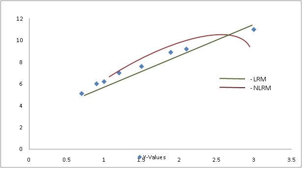
Considering Linear Regression Model (LRM)
From the formulas of $a$ and $b$ given above we get
$a = 0.78$ and $b = 0.56$
Considering Non Linear Regression Model (NLRM)
Taking log both the side
The above equation can be written as $y' = a' + bx'$ where
From the formulas of $a$ and $b$ given above we get
$a' = loga$
$x' = logx$
While in the second method the non linear form of equation is represented in a linear format and then calibration is done for the new linear equation obtained. Few examples of such non linear equation are given below
| Equation | Derivation |
|---|---|
| $y = ab^x$ | Taking log both the side $logy = loga + xlogb$ Thus new linear equation obtained is, $y' = a' + b'x$ |
| $y = ax^b$ | Taking log both the side $logy = loga + blogx $ Thus new linear equation obtained is, $y' = a' + bx'$ |
| $y = \dfrac{1}{(a+bx)}$ | Taking reciprocal of the equation we get $ \dfrac{1}{y} = a + bx $ Thus new linear equation obtained is, $y' = a + bx$ |
The solution for SLRM can be obtained from the procedure above. You can perform experiments not only on SLRM but also on MLRM and Non linear Models since it is tedious to work on them manually.
The Non Linear Models are
- Quadratic
- Power eg $(y\ =\ a_0x_0^{b_0}\ +\ a_1x_1^{b_1}+\ ....)$
- Exponential eg $(y\ =\ a_0e_0^{x_0}\ +\ a_1e_1^{x_1}+\ ....)$
- Logarithmic eg $(y\ =\ a_0\ +\ a_1 ln(x_0)\ +\ a_2 ln(x_1)+\ ....)$
Regression Analysis will give a relation between the trip production (attraction) and its relevant independent variables. This relationship can be assumed to continue for futuristic scenario. Thus by obtaining future census data of variables we can get future Production Attraction table.
To get an idea you can perform experiment by default file which is recent census data of Pune city.
ExamplePlanners have estimated the following models for the AM Peak Hour
$T_i=1.5*H_i$
$T_j=(1.5*E_{off,j})+(1*E_{oth,j})+(0.5*E_{ret,j})$
where,
$T_i$ = Person trips originating in zone $i$.
$T_j$ = Person trips destined in zone $i$.
$H_i$= Number of House holds in zone $i$
You are also given the following data
| Variable | City1 | City2 |
|---|---|---|
| H | 10000 | 15000 |
| Eoff | 10000 | 15000 |
| Eoth | 10000 | 15000 |
| Eret | 10000 | 15000 |
A. What are the number of person trips originating in and destined for each city?
B. Normalize the number of person trips so that the number of person trip origins = the number of person trip destinations.
SolutionA. The number of person trips originating in and destined for each city:
| Households (Hi) | Office Employees (Eoff) | Other Employees (Eoth) | Retail Employees (Eret) | Origins Ti = 1.5 * Hi | Destinations Tj = (1.5 * Eoff,j) + (1 * Eoth,j) + (0.5 * Eret,j) | |
|---|---|---|---|---|---|---|
| City1 | 10000 | 8000 | 3000 | 2000 | 15000 | 16000 |
| City2 | 15000 | 10000 | 5000 | 1500 | 22500 | 20750 |
| Total | 25000 | 18000 | 8000 | 3000 | 37500 | 36750 |
B. Normalize the number of person trips so that the number of person trip origins = the number of person trip destinations. Assume the model for person trip origins is more accurate. Use:
$$ \nonumber T'_j\ =\ T_j\dfrac{\sum\limits_{i=1}^I T_i}{\sum\limits_{j=1}^J T_j} = Tj\dfrac{37500}{36750} = T_j*1.0204 $$
| Originss (Ti) | Destinations (Tj) | Adjustment Factor | Normalized Destinations (Tj) | Rounded | |
|---|---|---|---|---|---|
| City1 | 15000 | 16000 | 1.0204 | 16326.53 | 16327 |
| City2 | 22500 | 20750 | 1.0204 | 21173.47 | 21173 |
| Total | 37500 | 36750 | 1.0204 | 37500 | 37500 |
References Books
- J. De D. Ortuzar and L.G. Willumsen (1996), Modelling Transport. Wiley Publications, London.
- C. S. Papacostas and P. D. Prevedouros (2001), Transportation Engineering & planning. Prentice-Hall of India, New Delhi.