Theory

Introduction

Calibration is an important step as it estimates the value of c in the gravity equation given below such that the model best fits the base year observations. Thus proper value of c fixes the relationship between the travel time factor and the interzonal impedance. Initially a value of c is assumed and applied using a base year observation of production, attraction and impedance to compute interzonal volumes which are then compared with the observed volume of the base year condition. If the value obtained of c gives close to the observed value then it can be used otherwise its value is changed and further iteration is done. Iteration is carried until sufficient convergence value of c is obtained. For calibration generally friction factor F is used rather than parameter c.

$$\nonumber T_{ij} = K \dfrac{P_i A_j}{W_{ij}^c}$$ Let, $\nonumber F_{ij} = K \dfrac{1}{W_{ij}^c}$
$\nonumber F_{ij}$=Friction Factor $$\nonumber T_{ij} = P_i F_{ij} \dfrac{A_j}{\sum \limits_{j}F_{ij} A_j}$$

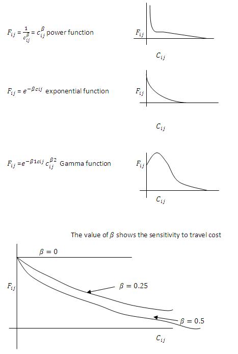
The comparison between the computed and the observed values is done with the help of trip length frequency distribution curve. Its a graphical relationship between the percentages of the region wide trips versus their interzonal impedance (example: time etc). The calibration of Gravity Model mainly depends on the assumed Friction Factor mathematical function. Some of the commonly used functions are shown below.

$\nonumber F_{ij} = t_{ij}^\beta$(Polynomial Function)

$\nonumber F_{ij} = e^{\beta t_{ij}}$ (Exponential Function)

$\nonumber F_{ij} = t_{ij}^\beta e^{\beta t_{ij}}$ (Two Parameters)

$\nonumber F_{ij} = $Discontinuous Function (BPR)

Examples of the above equations are given below.

Diagram

If the calibration is correct the observed and the simulated calculations will match but if they donot then a set of values of Friction Factor is calculated using the following expression:

$$\nonumber F' = F \dfrac{OD\%}{GM\%} $$

F^' = Friction factor to be used in next iteration

F = Friction used in calibration just completed

OD% = Percentage of total trips occuring for a given travel time observed in a travel survey

GM% = Percentage of total trips occuring for a given travel time obtained from Gravity model

This iteration is carried on till the trip length frequency curve of the observed and calculated value is obtained. The final phase of calibration procedure includes the calculation of zone to zone adjustment factor.

$$\nonumber k_{ij} = r_{ij}[ \dfrac{(1-x_i)}{(1-x_i r_{ij})}] $$

$ k_{ij}$ = Adjustment factor applied to movements between zone i and j

$ r_{ij}$ = (number of trips obtained from OD survey ) / (number of trips obtained from gravity model)

$ x_{i}$ = (Number of trips obtained from OD survey) / $ p_{i}$

The mathematical models used for Trip Distribution Model are as follows:

Calibration of single constrained gravity model
Calibration of doubly constrained gravity model

Calibration of Singly Constrained Gravity Model The steps involved for calibration of doubly constraint model is given below:

Assume a trial value of β.
Constraint any one either Trip Production (Origin) or Trip Attraction (Destination), suppose Origin is constraint (Remember: constraint is with respect to future trips).
A mathematical function that is selected in order to find the friction factor is calculated.
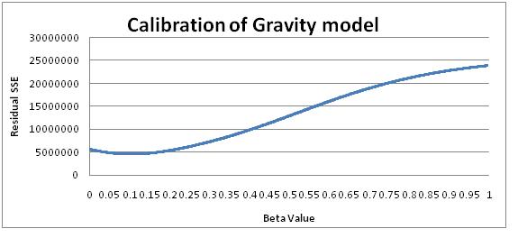
These values are substituted in the gravity model, the calculated destination values are compared with the future values, and the error between the two is calculated with the help of Residual Standard Square of Errors.
This error is minimised for an optimised value of β.
At the end of the calibration we get an optimised value of β.

Example

Calibration of Singly Constrained Gravity Model (Origin)

Cost Matrix
Zone	1	2	3
1	28	23	28
2	29	26	27
3	31	31	20

Given Trip Matrix
Zone	1	2	3	∑ [O_i]
1	3413	126	231	3770
2	151	564	729	1444
3	435	289	1806	2530
∑ [D_j]	3999	979	2766

Selected Frictional Functions: Exponential Function $\nonumber F_{ij} = e^{-\beta c_{ij}} $

Trip Matrix with respect to Optimal Beta Value (Minimum SSE)
Zone	1	2	3
1	1794	735	1240
2	661	220	562
3	745	182	1601

Minimum Residual = 4567836.6438594
Optimal Beta = 0.103

Target O_i	Modelled O_i	Target D_j	Modelled D_j
3770	3770	3999	3201.193385
1444	1444	979	1138.173227
2530	2530	2766	3404.633388

Diagram

References Books

J. De D. Ortuzar and L.G. Willumsen (1996), Modelling Transport. Wiley Publications, London.
C. S. Papacostas and P. D. Prevedouros (2001), Transportation Engineering & planning. Prentice-Hall of India, New Delhi.

Calibration of Singly Constrained Gravity ModelTrip Distribution

Theory