Transportation Network Design

Dr. Tom V. Mathew

Contents

• 1 Introduction
• 2 Traffic assignment
  • 2.1 All-or-nothing assignment
  • 2.2 Incremental assignment
  • 2.3 Capacity restraint assignment
  • 2.4 User equilibrium assignment (UE)
  • 2.5 System Optimum Assignment (SO)
  • 2.6 Example 1
  • 2.7 Example 2
  • 2.8 Stochastic user equilibrium assignment
  • 2.9 Dynamic Assignment
  
  
• 3 Limitation of conventional assignment models
• 4 Bilevel
• 5 Examples of Bilevel
  • 5.1 Network Capacity Expansion
  • 5.2 Combined traffic assignment and signal control
  • 5.3 Optimising Toll
  • 5.4 Formal Notation
  
  
• 6 Formulation of capacity expansion problem
• 7 Numerical Example
  • 7.1 Input
  • 7.2 Output
  • 7.3 Discussion
  
  
• Bibliography

1 Introduction

This document discusses the aspects of network design.First a brief introduction of network design will be given.Then various types of assignment techniques will be discussed including the mathematical formulation and numerical illustration of the important ones.Then the concept of bilevel programming and few examples will be presented.Finally one such example, namely the network capacity expansion will be formulated as a bilevel optimization problem and will be illustrated using a numerical example.

Transportation network design in a broad sense deeds with the configuration of network to achieve specified objectives.There are two variations to the problem, the continuous network design and the discrete network design. Examples of the form include

a

The determination of road width.

b

The calculation of signal timings.

c

The setting of road user charges.

Although this document covers the continous network design in detailed, basis underlinig principles are some form the discrete case. Conventional network design has been concerned with minimization of total system cost.However, this may be unrealistic in the sense that how the user will respond to the proposed changes is not considered. Therefore, currently the network designis thought of as supply demand problem or leader-follower game.The system designer leads, taking into account how the user follow. The core of all network design problems is how a user chooses his route of travel. The class of traffic assignment problem tries to model these behaviour. Therefore, the traffic assignment will be discussed before adressing bi-level formulation of the network design problems.

2 Traffic assignment

The process of allocating given set of trip interchanges to the specified transportation system is usually refered to as traffic assignment. The fundamental aim of the traffic assignment process is to reproduce on the transportation system, the pattern of vehicular movements which would be observed when the travel demand represented by the trip matrix, or matrices ,to be assigned is satisfied. The major aims of traffic assignment procedures are:

1. To estimate the volume of traffic on the links of the network and possibly the turning movements at intersections.
2. To furnish estimates of travel costs between trip origins and destinations for use in trip distribution.
3. To obtain aggregate network measures, e.g. total vehicular flows, total distance covered by the vehicle, total system travel time.
4. To estimate zone-to-zone travel costs(times) for a given level of demand.
5. To obtain reasonable link flows and to identify heavily congested links.
6. To estimate the routes used between each origin to destination(O-D) pair.
7. To analyse which O-D pairs that uses a particular link or path.
8. To obtain turning movements for the design of future junctions.

The types of traffic assignment models are all-or-nothing assignment, incremental assignment, capacity restraint assignment, user equilibrium assignment (UE), stochastic user equilibrium assignment (SUE), system optimum assignment (SO), etc. These frequently used models are discussed here.

2.1 All-or-nothing assignment

In this method the trips from any origin zone to any destination zone are loaded onto a single, minimum cost, path between them. This model is unrealistic as only one path between every O-D pair is utilised even if there is another path with the same or nearly same travel cost. Also, traffic on links is assigned without consideration of whether or not there is adequate capacity or heavy congestion; travel time is a fixed input and does not vary depending on the congestion on a link. However, this model may be reasonable in sparse and uncongested networks where there are few alternative routes and they have a large difference in travel cost. This model may also be used to identify the desired path : the path which the drivers would like to travel in the absence of congestion. In fact, this model's most important practical application is that it acts as a building block for other types of assignment techniques.It has a limitation that it ignores the fact that link travel time is a function of link volume and when there is congestion or that multiple paths are used to carry traffic.

2.2 Incremental assignment

Incremental assignment is a process in which fractions of traffic volumes are assigned in steps.In each step, a fixed proportion of total demand is assigned, based on all-or-nothing assignment. After each step, link travel times are recalculated based on link volumes. When there are many increments used, the flows may resemble an equilibrium assignment ; however, this method does not yield an equilibrium solution. Consequently, there will be inconsistencies between link volumes and travel times that can lead to errors in evaluation measures. Also, incremental assignment is influenced by the order in which volumes for O-D pairs are assigned, raising the possibility of additional bias in results.

2.3 Capacity restraint assignment

Capacity restraint assignment attempts to approximate an equilibrium solution by iterating between all-or-nothing traffic loadings and recalculating link travel times based on a congestion function that reflects link capacity. Unfortunately, this method does not converge and can flip-flop back and forth in loadings on some links.

2.4 User equilibrium assignment (UE)

The user equilibrium assignment is based on Wardrop's first principle, which states that no driver can unilaterally reduce his/her travel costs by shifting to another route. If it is assumed that drivers have perfect knowledge about travel costs on a network and choose the best route according to Wardrop's first principle, this behavioural assumption leads to deterministic user equilibrium. This problem is equivalent to the following nonlinear mathematical optimization program,

$${\mathrm Minimize  }Z = \sum_{a}\int_0^{x_{a}}t_{a}(x_{a})dx,$$ (1)

$${\mathrm subject  to  } \sum_{k}f_k^{rs} = q_{rs} :\forall r,s$$

$$x_a = \sum_r \sum_s \sum_k \delta_{a,k}^{rs}f_k^{rs} :\forall a$$

$$f_k^{rs} \geq 0 : \forall  k,r,s$$

$$x_a \geq 0 : a \in A$$

k is the path, $x_a$ equilibrium flows in link a, $t_a$ travel time on link a,  $f_k^{rs}$ flow on path k connecting O-D pair r-s, $q_{rs}$ trip rate between r and s.

The equations above are simply flow conservation equations and non negativity constraints, respectively. These constraints naturally hold the point that minimizes the objective function. These equations state user equilibrium principle.The path connecting O-D pair can be divided into two categories : those carrying the flow and those not carrying the flow on which the travel time is greater than (or equal to)the minimum O-D travel time. If the flow pattern satisfies these equations no motorist can better off by unilaterally changing routes. All other routes have either equal or heavy travel times. The user equilibrium criteria is thus met for every O-D pair. The UE problem is convex because the link travel time functions are monotonically increasing function, and the link travel time a particular link is independent of the flow and other links of the networks. To solve such convex problem Frank Wolfe algorithm is useful.

2.5 System Optimum Assignment (SO)

The system optimum assignment is based on Wardrop's second principle, which states that drivers cooperate with one another in order to minimise total system travel time. This assignment can be thought of as a model in which congestion is minimised when drivers are told which routes to use. Obviously, this is not a behaviourally realistic model, but it can be useful to transport planners and engineers, trying to manage the traffic to minimise travel costs and therefore achieve an optimum social equilibrium.

$${\mathrm Minimize  }Z = \sum_{a} x_{a}t_{a}(x_{a})$$ (2)

$${\mathrm subject  to  } \sum_{k}f_k^{rs} = q_{rs} :\forall r,s$$

$$x_a = \sum_r \sum_s \sum_k \delta_{a,k}^{rs}f_k^{rs} :\forall a$$

$$f_k^{rs} \geq 0 : \forall  k,r,s$$

$$x_a \geq 0 : a \in A$$

$x_a$ equilibrium flows in link a, $t_a$ travel time on link a, $f_k^{rs}$ flow on path k connecting O-D pair r-s, $q_{rs}$ trip rate between r and s.

2.6 Example 1

To demonstrate how the most common assignment works, an example network is considered. This network has two nodes having two paths as links.

Let us suppose a case where travel time is not a function of flow as shown in other words it is constant as shown in the figure below.

Figure 1: Two Link Problem with constant travel time function

2.6.1 All or nothing

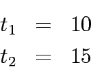
The travel time functions for both the links is given by:

$$\begin{eqnarray*} t_1 &=& 10\\ t_2 &=& 15 \end{eqnarray*}$$

and total flows from 1 to 2.

$$\begin{eqnarray*} q_{12} &=& 12 \end{eqnarray*}$$

Since the shortest path is Link 1 all flows are assigned to it making $x_1^*$ =12 and $x_2^*$ = 0.

2.6.2 User Equilibrium

Substituting the travel time in equations 1 - 5 yield to

$$\begin{eqnarray*} min:   Z(x)&=& \displaystyle\int^{x_1}_0 10 dx_1 + \int^{x_2}_0 15 dx_2 \\ &=& 10x_1 + 15x_2 \\ st:   x_1 + x_2 &=& 12. \end{eqnarray*}$$

Substituting $x_2= x_1-12$, in the above formulation will yield the unconstrained formulation as below :

$$\begin{eqnarray*} min Z(x)&=&10x_1 + 15(12-x_1) \end{eqnarray*}$$

Differentiate the above equation w.r.t $x_1$ and equate to zero, and solving for $x_1$ and then $x_2$ leads to the solution $x_1^*$ = 12, $x_2^*$ = 0.

2.6.3 System Optimization

Substituting the travel time in equation: (6-8), we get the following:

$$\begin{eqnarray*} min:  Z(x) &=& {x_1}\times({10}) + {x_2}\times({15}) \\ & =& 10{x_1} + 15{x_2} \end{eqnarray*}$$

Substituting $x_2= 12- x_1$ the above formulations takes the following form:

$$\begin{eqnarray*} min:   Z(x)&=&10{x_1} + 15{(12-x_1)} \end{eqnarray*}$$

Differentiate the above equation w.r.t $x_1$ and equate to zero, and solving for $x_1$ and then $x_2$ leads to the solution $x_1^*$ = 12, $x_2^*$= 0, and $Z(x^*)$ = 120.

2.6.4 Comparison of results

After solving each of the formulations the results are tabulated in Table 1. One can infer that if the travel time is independent of the flow, then essentially there in no difference between the various assignment types.

Table 1: Comparison of results for example 1

Type	$t_1$	$t_2$	$x_1$	$x_2$	$Z(x^*)$	TSTT
AON	10	15	12	0	120	120
UE	10	15	12	0	120	120
SO	10	15	12	0	120	120

2.7 Example 2

Figure 2: Two Link Problem with variable travel time function

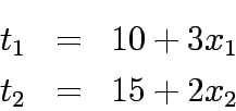
Lets now take a case where travel time functions for both the links is given by:

$$\begin{eqnarray*} t_1 &=& 10+3x_1\\ t_2 &=& 15+2x_2 \end{eqnarray*}$$

and total flows from 1 to 2.

$$\begin{eqnarray*} q_{12} &=& 12 \end{eqnarray*}$$

2.7.1 All or Nothing Assignment

Assume $x_1,x_2=0$ which makes $t_1=1$0 and $t_2=15$. Since the shortest path is Link 1 all flows are assigned to it making $x_1$ =12 and $x_2$ = 0.

2.7.2 User Equilibrium

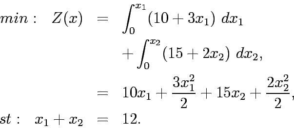
Substituting the travel time in equations 1 - 5 yield to

$$\begin{eqnarray*} min:   Z(x)&=& \int^{x_1}_0 (10+3x_1) dx_1\\ && + \int^{x_2}_... ...x_1^2}{2} + 15x_2 + \frac{2x_2^2}{2},\\ st:   x_1 + x_2 &=& 12. \end{eqnarray*}$$

Substituting $x_2= 12- x_1$, in the above formulation will yield the unconstrained formulation as below:

$$\begin{eqnarray*} min:  Z(x)&=& 10x_1 + \frac{3x_1^2}{2}, \\ && + 15(12-x_1) + \frac{2(12-x_1)^2}{2}. \end{eqnarray*}$$

Differentiate the above equation w.r.t $x_1$ and equate to zero, and solving for $x_1$ and then $x_2$ leads to the solution $x_1$ = 5.8, $x_2$ = 6.2.

2.7.3 System Optimization

Substituting the travel time in equation: (6-8), we get the following:

$$\begin{eqnarray*} min:  Z(x)&=& {x_1}\times({10+3x_1}) + {x_2}\times({15+2x_2}) \\ &=& 10{x_1}+3{x_1}^2 + 15{x_2}+2{x_2}^2 \end{eqnarray*}$$

Substituting $x_2= x_1-12$

$$\begin{eqnarray*} min:  Z(x) &=& 10{x_1}+3{x_1}^2\\ &+& 15{(12-x_1)}+2{(12-x_1)}^2 \end{eqnarray*}$$

Differentiate the above equation w.r.t zero, and solving for $x_1$ and then $x_2$ leads to the solution $x_1^*$ = 5.3, $x_2^*$= 6.7, and $Z(x^*)$ = 327.55.

2.7.4 Comparison of results

After solving each of the formulations the results are tabulated in Table 2. One can infer that unlike earlier, the various assignment types shows considerable differences in the performace. AON has obviously the worst solution and SO has the best.

Table 2: Comparison of results for example 2

Type	$t_1$	$t_2$	$x_1$	$x_2$	$Z(x^*)$	TSTT
AON	10	15	12	0	467.44	552
UE	27.4	27.4	5.8	6.2	239.0	328.8
SO	30.1	25.6	5.3	6.7	327.5	327.5

2.8 Stochastic user equilibrium assignment

User equilibrium assignment procedures based on Wardrop's principle assume that all drivers percieve costs in an identical manner. A solution to assignment problem on this basis is an assignment such that no driver can reduce his journey cost by unilaterally changing route. Van Vilet considered as stochastic assignmnet models, all those models which explicitly allows non minimum cost routes to be selected. Virtually all such models assume that drivers perception of costs on any given route are not identical and that the trips between each O-D pair are divided among the routes with the most cheapest route attracting most trips. They have important advantage over other models because they load many routes between individual pairs of network nodes in a single pass through the tree building process,the assignments are more stable and less sensitive to slight variations in network definitions or link costs to be independent of flows and are thus most appropriate for use in uncongested traffuc conditions such as in off peak periods or lightly trafficked rural areas.

2.9 Dynamic Assignment

Dynamic user equilibrium,expressed as an extension of Wardrop's user equilibrium principle, may be defined as the state of equilibrium which arises when no driver an reduce his disutility of travel by choosing a new route or departure time,where disutility inclues, schedule delay in addition in to costs generally considered. Dynamic stochastic equilibrium may be similarly defined in terms of percieved utility of travel. The existence of such equilibria in complex networks has not been proven theoretical and even if they exist the question of uniqueness remains open.

3 Limitation of conventional assignment models

The specific limitations of the assignment models are highlighted below.

1. Most of the cost functions, such as the BPR function, do not take into consideration emission-related factors.
2. Interactions between links are not considered; the travel time on one link is independent of the volumes on other links. This is an obvious oversimplification. At intersections, link travel times are affected by volumes on other approaches and opposing left turns. On freeways, merging and weaving conditions can greatly affect travel times. Queuing caused by bottlenecks on other links can also be a factor. Queues build as volumes approach the bottleneck
3. Although some software packages allow node-based capacities, delays, or performance functions which allows for better modeling of intersection dynamics. However, many of the problems described above cannot be eliminated through network solutions. Some of these issues can be addressed by considering the effects of flows on other links and the delays at a junction, on the link under investigation.

4 Bilevel

The bilevel programming (BLP) problem is a special case of multilevel programming problems with a two level structure. The problem can be expressed as follows: the transport planner, wishes to determine an optimal policy as a function of his or control variables (y) and the users response to these controls, where users response generally takes the form of a network flow (x). The transport planner then seeks to minimise a function of both y and x, where some constraints may be imposed upony as well as the fact that x should be a user equilibrium flow, parameterised by the control vector,y. There exists many problems in transportation that can be formulated as bilevel programming problem.They include network capacity expansion, network level signal setting and optimum toll pricing. They are discussed briefly here:

5 Examples of Bilevel

5.1 Network Capacity Expansion

The network capacity expansion problem is to determine capacity enhancements of existing facilities of a transportation network which are, in some sense, optimal. Network design models concerned with adding indivisible facilities (modeled as integer variables) are said to be discrete, whereas those dealing with divisible capacity enhancements (modeled as continuous variables) are said to be continuous. Thus network expansion problem is a continuous network design problem,which determines the set of link capacity expansions and the corresponding equilibrium flows for which measures of performance index for network is optimal. A bilevel programming technique can be used to formulate this equilibrium network design problem. At the upper level problem, the system performance index is defined as the sum of total travel times and investment costs of link capacity expansions. At the lower level problem, the user equilibrium flow is determined by Wardrop's first principle and can be formulated as an equivalent minimization problem. The most well-studied equilibrium network design problem is user equilibrium network design with fixed transportation demand.

5.2 Combined traffic assignment and signal control

For a road network with flow responsive signal control and fixed origin-destination travel demands. Combined traffic assignment and signal control problem tries to allocate the demand matrix to the network subject to user equilibrium assumption and computes the optimal signal control parameter from the generated link flows.Consider f and g, which denote respectively, a vector of link flows and a vector of signal settings for the network; assuming that the signal plan structure is given (specified by number, type, and sequence of phases), signal settings may consist of cycle length's, green splits, and offsets.Traffic equilibrium,${\bf {x}}^{*}$ is a set of link flows satisfying satisfying Wardrop's first principle.

The equilibrium traffic signal setting is a pair $(\bf {x}^{*},\bf {s}^{*})$ such that $\bf {x}^{*}$ is a traffic equilibrium when signals are set at $\bf {s}^{*}$.

$${\bf {x}}^*={\bf {f}}^e({\bf {s}}^*)$$ (3)

where ${\bf {s}}^{*}$ is the signal settings corresponding to ${\bf {x}}^{*}$ under specified control policy P;

$$\bf {s}^*={\bf {g}}^p({\bf {x}}^*)$$ (4)

If there exists a pair $({\bf {x}}^{*}, {\bf {s}}^{*})$, then link flows and signal settings are

$${\bf {x}}^*={\bf {f}}^e\lbrack {\bf {g}}^p({\bf {x}}^*)\rbrack or {\bf {g}}^*={\bf {g}}^p\lbrack {\bf {f}}^e({\bf {s}}^*)\rbrack$$ (5)

5.3 Optimising Toll

In general,traffic flow and queue size on a road network depend on road toll pattern and also traffic control. An efficient pricing scheme should therefore take into account the effects of the altered network flow pattern and queueing due to road pricing to achieve a global optimal solution. This requires development of an efficient procedure for calculating optimal toll patterns in general road networks while anticipating driver response in terms of route choice. The procedure should be able to estimate queueing delay and queue length, both of which are critical in queue management in congested urban road networks. Optimum toll pricing problem can be formulated as a bilevel programming in general road networks. The users route choice behaviour under condition of queing and congestion in a road network for any given toll pattern can be represented by the mathematical programming model.Global evaluation of likely effects of road pricing thud becomes possible.The model can be formulated to find an optimal set of link tolls such that a particular system performance criterion is optimized.A meaningful objective is to optimize is to minimize the total network cost or to maximize total revenue raised from toll charges. In this kind of problem,it is assumed that for any given toll pattern,u,there is a unique equilibrium flow distribution,x,obtained from the lower-level problem. x is also called the response or reaction function. An efficient toll pattern,u, will greatly depend on how to evaluate the reaction function x, or in other words,how to predict route changes of users in response to alternative toll charges. This interaction game can be represented as the following bi-level programming problem:
Lower Level:

$${\bf {x}}^*={\bf {f}}^e({\bf {u}}^*)$$ (6)

where ${\bf {u}}^*$ is the signal settingd corresponding to ${\bf {x}}^*$ under specified control policy P;

$${\bf {u}}^*={\bf {g}}^e({\bf {x}}^*)$$ (7)

If there exists such a pair ${(x^*,u^*)}$, then link flows and signal settings are

$${\bf {x}}^*={\bf {f}}^e\lbrack {\bf {g}}^p({\bf {x}}^*)\rbrack or {\bf {g}}^*={\bf {g}}^p\lbrack {\bf {f}}^e({\bf {s}}^*)\rbrack$$ (8)

There can be be three types of formulation on upper level, one is total network travel cost $F_1$, the sum of travel times and queueing delays experienced by all vehicles:

$$F_1 = {\sum_{a \in A}} {v_at_a(v_a)+v_ad_a}$$ (9)

The total revenue, denoted as $F_2$, arising from toll charges can be expressed as:

$$F_2 = {\sum_{a \in A^{\ast}}}{u_a}{v_a}$$ (10)

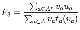
A third objective function can be to maximize the ratio, denoted as $F_3$, of the total revenue to total cost :

$$F_3 = \frac {\sum_{a\in A^{\ast}} v_au_a} {\sum_{a\in A} {v_a}{t_a(v_a)}}$$ (11)

where $u_a$ is travel cost $v_a$ is exit flows and $d_a$ are the queueing delay.

5.4 Formal Notation

Consider a road network and suppose that origin destination travel demand is fixed and known. Let x and y denote respectively vector of link flows and a vector of network expansion policy. A Budget control policy, denoted by B is in general any rule or procedure that can be used to determine the components of 'y' when 'x' is known. The network design problem consists of finding a pair $(x^\ast,y^\ast)$,such that $x^\ast$ is at traffic equilibrium when capacity is $y^\ast$.

$$x^\ast = f^e (y^\ast)$$ (12)

where $y^\ast$ is the capacity improvement corresponding to a $x^\ast$ under specified Budget B and $f^e$ is the function that gives the vector of link flows.

$$y^\ast = g^P (x^\ast)$$ (13)

where $g^P$ is a function that given optimal capacity expansion vector for a given $x^*$. If there exists such a pair ($x^\ast$,$y^\ast$ ) then link flows and capacity improvement are mutually consistent or in equilibrium , in the sense that users choice when controls are at $y^\ast$ yield link flows equal to those from which $y^\ast$ arises under budget constraint B.In other words

$$x^\ast = x^e [y^P (x^\ast )] \mid constant y$$ (14)

or equivalently

$$y^\ast = y^P [x^e(y^\ast )] \mid constant x$$ (15)

Figure 3: Bilevel

6 Formulation of capacity expansion problem

The following notation has been used for CNDP formulation:
Let A be the set of links in the network, $\Omega$ the set of OD pairs,  q the vector of fixed OD pair demands,q = ${q_{rs}}$,  K the set of paths between OD pair $\omega$, f the vector of path flows between OD pair r,s on path k which means f = [$f_k^{rs}$],  x the vector of link flows, x = ${x_a}$, y the vector of link capacity expansion,  y = ${y_a}$, B the allocated budget for expansion, $t_a$ travel time on link a,  $\gamma_a$ is the coefficient of link expansion vector y,, $f_k^{rs}$ flow on path k connecting O-D pair r-s,  $q_{rs}$ trip rate between r and s.

Upper Level

$$min Z{(x)} = \sum_{\forall a} x_at_a(x_a,y_a)$$ (16)

subject to

$$\sum_{\forall a}\gamma_ay_a \leq B$$ (17)

$$y_a\geq 0 : \forall a \in A$$ (18)

Lower Level

$$min Z(x)= \sum_{\forall a}\displaystyle\int^{x_a}_0 t_a(x_a) ds$$ (19)

subject t

$$\sum_{\forall k}f_k^{rs}=q_{rs} :k\in K;r,s\in \Omega$$ (20)

$$x_a = \sum_r \sum_s \sum_k \delta_a,k^{rs}f_k^{rs} :a \in A;k\in K$$ (21)

$$f_k^{rs} \geq 0 : r,s \in Omega;k\in K$$ (22)

$$x_a \geq 0 : a \in A$$ (23)

$x_a$ equilibrium flows in link a, $t_a$ travel time on link a, $y_a$ link capacity expansions in link a, $\gamma_ay_a$, $f_k^{rs}$ flow on path k connecting O-D pair r-s, $q_{rs}$ trip rate between r and s. To illustrate how the bilevel problem of network capacity expansion works an example network was considered.This network had four nodes and five links.Two links were considered for improvement. The figure shows the network.

7 Numerical Example

Figure 4: Bilevel example problem

7.1 Input

$$q_{23} = 50$$ (24)

$$q_{03} = 80$$ (25)

$$t = t_o \left(1+ \alpha (\frac{x}{K})^\beta \right)$$ (26)

$$B = 10$$ (27)

From	To	$\alpha$	$\beta$	length(Km)	Capacity(K)	Speed(Km/hr)
1	2	0.15	4.0	1.0	20.0	60.0
1	3	0.15	4.0	1.0	20.0	60.0
2	4	0.15	4.0	1.0	30.0	60.0
3	2	0.15	4.0	1.0	30.0	60.0
3	4	0.15	4.0	1.0	40.0	60.0

7.2 Output

no.	x0*	x1*	x2*	x3*	x4*	UE	TSTT	z1*	z2*	SO
1	42.5	38.71	52.87	10.37	79.09	317.39	692.8	5.36	4.64	609.41
2	38.78	42.27	56.05	17.27	75.65	296.85	564.23	5.79	4.21	564
3	38.61	42.44	55.67	17.06	76.02	296.73	564.48	5.95	4.05	564.45
4	38.45	42.56	55.58	17.13	76.07	296.53	563.5	6.02	3.98	563.5
5	38.51	42.53	55.48	16.97	76.21	296.68	564.61	6.04	3.96	564.61
6	38.5	42.53	55.46	16.96	76.22	296.66	564.6	6.04	3.96	564.6

7.3 Discussion

The initial link expansion vector is taken as 0. User equilibrium is performed to get the required link flows. Now these flows are input to upper level from where we get a new set of link expansion vectors which minimizes the system travel time.This iteration is repeated until the total sytem travel time from lower level and upper level converges.

Bibliography

1

Y. Sheffi, Urban transportation networks: Equilibrium analysis with mathematical programming methods.
New Jersey: Prentice-Hall, 1984.

2

R. Thomas, Traffic Assignment Techniques.
England: Avebury Technical publication, 1991.